362

"Rollover B8 OV1" (like Rollover Beethoven...? get it?)

Update 17 July 2011: This blog entry was featured in Chandoo's latest post. So if you're coming here from his site -- welcome!

original post:

This post was inspired by Chandoo's post on hyperlinks in Excel. If you haven't checked his website out yet - you should. It's excellent.

In this post, I suggest a method for creating a "Rollover" effect for your mouse on an Excel spreadsheet. Rollover techniques (also called "Mouseovers") are useful to (1) display quick information to the user; (2) to execute a function when a user puts their mouse over a specific region; and (3) to make neat graphical effects.

For item 1, my technique isn't really necessary. If you want to display brief information to the user when he or she rolls over a cell, the best way to do this is to insert a comment.

But comments are pretty limited. You can only write so much information in a comment before it becomes too cluttered to be useful. Moreover, comments are static. What if you want the information concerning the "target" cell (that is, the cell to be rolled over) to change based on different items in your spreadsheet? We can use the in-cell Hyperlink() formula to accomplish this.

The Hyperlink() formula looks like this:

=Hyperlink(location, [Friendly Text])
location - Here you write the intended address of your hyperlink. This can be a webpage (i.e. "http://www.google.com") or a file on your computer.
[Friendly Text] - This is an optional field that provides a caption to your hyperlink. If you leave it blank, it will simply display the address in the previous parameter.

To begin our example, you'll need to create a User Defined Function (UDF) to be executed when the rollover event is initiated. So go into the Visual Basic Environment, create or find a free module and create a UDF that looks something like this.

Public Function MyMouseOverEvent()

Sheet1.Range("A1").Value = "Event Fired!"

End Function

I can understand if you're puzzled at this point. UDFs are not really allowed to change values in other cells. However, since we'll be calling this function from within the Hyperlink() formula, you'll see this limitation no longer exists.

So now go to Sheet1 and click on cell A2. In that cell, type in the following formula:

=HYPERLINK(MyMouseOverEvent(),"Click here")

Upon hitting Enter, you should get a #VALUE! error, but ignore it for a second. Roll your mouse over cell A2 - and viola! - Cell A1 should now say "Event Fired!"

But what about that pesky #VALUE! error? Remember the limitation that UDFs can't change other cells? Well, even though Excel let's you change a value from within your UDF, it still recognizes that it wasn't supposed to! To get rid of that error is pretty simple. Just rewrite the function in your cell as follows:

=IFERROR(HYPERLINK(MyMouseOverEvent(),"Click here"), "Click here")

And that's it. If you like this technique and find some cool uses for it, drop me an email and show me.

Here's some graphical fun I created using this technique. Putting the mouse inside the black rectangle creates a fading snake-like pattern based on your mouse movements. Check out the screen capture:

Make sure to check out my latest (and greatest) example of this technique, here:

Periodic Table of Elements in Excel: Rollover Edition!

Author: Unknown Labels: Dashboards, Dynamic Charts, Excel Development, Interactive Dashboards, Spreadsheet Tricks, VBA

4

Sometimes, you'll want to programmatically take advantage of Windows outside the capabilities readily available through Visual Basic for Applications (VBA). For example, both eliminating the "Close"-button or creating a more opaque background on a window require the use of the Windows API.

Doing this in Visual Basic isn't too hard, but there are some distinct differences between what's readily available to programmers in Microsoft Office's Visual Basic (VBA) compared to its virtual twin, Visual Basic 6.0, and its smarter, object-oriented younger brother VB.net. Specifically, UserForms in VBA do not contain methods to find their Windows handle, (aka, their hWnd).

And most window modifying APIs require the target window's handle. Luckily, the Windows API also contains a function to find a given window's hWnd, called FindWindow():


Public Declare Function FindWindow Lib "user32" Alias "FindWindowA" _
(ByVal lpClassName As String, ByVal lpWindowName As String) As Long


So, to find your window's handle, you'll do something like this (assuming you're coding within the UserForm).


hWnd = FindWindow("ThunderDFrame", me.caption)


Here, FindWindow() takes two arguments. First, the class name of the window for which you're searching; and second, the window's caption.

ThunderDFrame, huh?

I know, right? The UserForms in Excel are actually of the Windows class ThunderDFrame, which is the class for all UserFroms in Microsoft Office applications after 2002 (it was "ThunderXFrame" before that). I've looked online for a good explanation for the name but haven't really found anything. Either way you'll need to pass that into the first argument of FindWindow whenever you need a UserForm's handle.


That's all for now!

-

ps I'm working on a better stylesheet for when I display code.

Author: Unknown Labels: FindWindow, VBA, Windows API

0

Excel really doesn't have an explicit "between function" to allow users, given a set of ranges, to find in what range a selected number falls. The obvious and messy workaround is to use a bunch of nested IFs, which is tedious and error-prone. That's where the RANK function comes in.

Here's a breakdown.

RANK(number,ref,[order])
number - The number you want to find
ref - The reference to spreadsheet range
order - optional; excel defaults to descending order

The RANK function returns the location of a specified number in a given range. So let's say you have a given set, 1,2,3,4,5. Obviously, testing for the number three will return a location of 3. For our range test, we combine a number outside the set and see where it falls.

Check out the image below to see it in action:


Excel returns a rank of 4, since 3.2 will appear in the fourth location of the ranked set, 1,2,3,3.2,4,5.
At this point, there are two important items to point out.

• How excel sorts the data for ranking is important. Above we use an ascending order (we pass a 1 to the last argument) and below we'll use a descending order (we'll pass a 0 to the last argument). You'll have to decide which best fits your analysis.
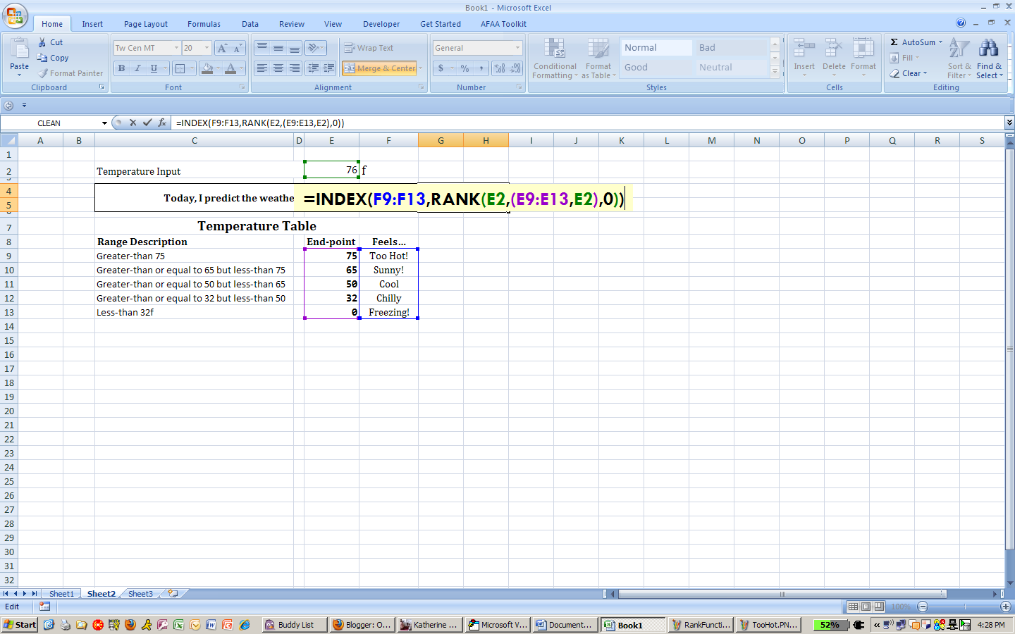
• Because you combine two ranges into one, you must use parenthesis. If you miss this step, the RANK function will interpret B2 as the next parameter and return an error.

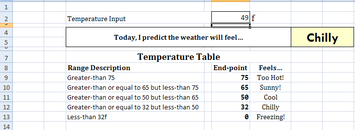
Here's a Weather Application



This example tests for a temperature's range and then displays how the day will feel corresponding to that range.

-

You could also use this trick when you must evaluate a value on a complex function. For example, you might have a graph with several curves that represents some utility for a given value, x. Thus, if you know the bounds of your curves, you can test in what range your x falls and apply its corresponding curve-function.

Finally, you might have noticed that this trick restricts you to inequalities with an inclusive lower bound and exclusive upper bound. There's ways to fix this and I plan to talk more about them in future posts.

Author: Unknown Labels: Excel Math, Formulas, Lookups, Rank()