Everyone! We've moved to WordPress.

Gangnam Cell Styles...Delete

0
A reader on one of the LinkedIn Excel Groups recently asked how to delete cell styles from a workbook. Today, I'll show a possible solution.

The Cell Styles Group:


List Cell Styles:

I opened a workbook, Alt+F11 for the Visual Basic Editor and cooked up the code below. I then opened another workbook and made sure the first sheet was active by clicking on cell $A$1.

I then ran this code:

1:  Option Explicit
2:  Sub ListStyles()
3:    'List all styles in a workbook

4:    Dim C As Range
5:    Dim rng As Range
6:    Dim i As Long
7:    Dim lRows As Long

8:    With Application
9:      .ScreenUpdating = False
10:      .EnableEvents = False
11:    End With

12:    With ActiveWorkbook
13:      'Add a temporary sheet
14:       .Sheets.Add before:=Sheets(1)
15:      'List all the styles
16:       For i = 1 To .Styles.Count
17:        ActiveSheet.Cells(Rows.Count, 1).End(xlUp).Offset(1, 0) = _
18:          .Styles(i).Name
19:      Next i
20:    End With

21:    'Tidy up
22:     'Destroy objects
23:     Set rng = Nothing
24:     Set C = Nothing
25:     'Excel environment
26:     With Application
27:      .DisplayAlerts = True
28:      .EnableEvents = True
29:     End With
30:  End Sub  

This returned 47 different styles. I am not going to list them all here. They are included in the workbook that you may download at the end of the post. Your workbook may have more or less depending on any customizations you have already made to your workbook or if you are working on a workbook you received from someone else.

Once you have a list of the styles, you may edit the list for thes styles you wish to keep or leave them all on the list if you wish to delete them all.

Let's see what happens if we delete all of them, shall we? This will only impact Cell Styles. It will not impact Table Styles or Chart Styles.

Styles Group Before Delete:


Delete Cell Styles:

Here's the code I am going to use to delete all cell styles from the cell styles group.

1:  Option Explicit
2:  Sub ClearStyles()
3:    'Deletes all styles from the active workbook
4:    Dim lRows As Long
5:    Dim C As Range
6:    Dim rng As Range

7:    With Application
8:      .ScreenUpdating = False
9:      .EnableEvents = False
10:      .DisplayAlerts = False
11:    End With

12:    'Make sure to click on sheet with list of styles to be deleted
13:    'Assumes list begins in $A$1
14:     With ActiveSheet
15:      lRows = .Cells(Rows.Count, 1).End(xlUp).Row
16:      Set rng = Range(.Cells(1, 1), Cells(lRows, 1))
17:     End With

18:    With ActiveWorkbook
19:      For Each C In rng
20:        On Error Resume Next
21:        .Styles(C.Text).Delete
22:        .Styles(C.NumberFormat).Delete
23:      Next C
24:    End With

25:    'Tidy up
26:     'Destroy objects
27:     Set rng = Nothing
28:     Set C = Nothing
29:     'Excel environment
30:     With Application
31:      .ScreenUpdating = True
32:      .DisplayAlerts = True
33:      .EnableEvents = True
34:     End With
35:  End Sub

Bam!!


Deleted 46 out of 47. Apparently cannot delete all styles or at least the "Normal" style.

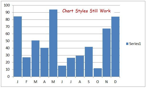
Chart styles still work


Excel Table styles still work


You may now add any custom styles to your workbook. But please, no Gangnam Style :-)
(Sorry Psi)


More on Styles and VBA from Jan Karlel Pieterse
Download the Cell Styles workbook here

How do you work with Cell Styles and VBA? Let us know in the comments section.


Are You Series(ous)?

0
Do you work with different series in your Excel charts?

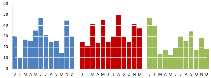
Here is what I would like the final chart to loo like. Note the white dashed lines in front of the columns:

Setup:

I started with the chart I ended with in my last post, Points Of Interest.


I then added some data to a separate worksheet in my workbook to replicate the horizontal gridlines.

The horizotal gridline scale is in units of 10, so I will use the same scale for my series' that I create for the "fake" gridlines.


Note in Col A that I used the exact same scale that I used for Series 1 which is what was used to plot the column charts (Really 1 chart)

Also note that I put data that is used for formatting on a separate worksheet from "Value Data". This makes it easier to maintain data as it needs to updated overtime


1. Horizontal gridlines

I am going to add fake horizontal gridlines to the chart, so first I'l remove the current horizontal gridlines.
  • Click on the chart (This will activate the Chart Tools Group on the Ribbon)
  • Click on "Layout" in the chart tools group
  • Click on gridlines
  • Click on Primary Horizontal Gridlines
  • Click on "None"


2. Add "Fake" horizontal gridlines

I copied all data from the formatting tab including the horizontal axis column, clicked on my chart and pasted the new series.

 I could click on each of the new series on the chart and change the chart type from column to line and apply all of the formatting. But I would like to do it with VBA. So I'll step through each part of the process separately
 

3. Change the chart type:

First I need to chage the chart type for each series that is not a value series which was series 1. So I'll loop through the SeriesCollection starting at number 2

1:  Option Explicit
2:  Sub SetChartType()
3:    Dim wb As Workbook
4:    Dim ws As Worksheet
5:    Dim i As Integer
6:    Set wb = ThisWorkbook
7:    Set ws = wb.Worksheets("Sheet1")
8:    With ws
9:      .ChartObjects(1).Activate
10:      For i = 2 To .ChartObjects(1).Chart.SeriesCollection.Count
11:        .ChartObjects(1).Chart.SeriesCollection(i).ChartType = xlLine
12:      Next i
13:    End With
14:    'Tidy up
15:      Set ws = Nothing
16:      Set wb = Nothing
17:  End Sub


4. Format the color of the lines

I would like each of the horizontal lines to be white

1:  Option Explicit
2:  Sub SetChartColor()
3:    Dim wb As Workbook
4:    Dim ws As Worksheet
5:    Dim i As Integer
6:    Dim lWhite As Long
7:    Set wb = ThisWorkbook
8:    Set ws = wb.Worksheets("Sheet1")
9:    lWhite = RGB(255, 255, 255)
10:    With ws
11:      .ChartObjects("Chart 1").Activate
12:      With ActiveChart
13:        For i = 2 To .SeriesCollection.Count
14:          .SeriesCollection(i).Select
15:          With Selection
16:            .Format.Line.ForeColor.RGB = lWhite
17:          End With
18:        Next i
19:      End With
20:    End With
21:    'Tidy up
22:      Set ws = Nothing
23:      Set wb = Nothing
24:  End Sub  


5. Change the line type:

The chart is looking pretty good. But the lines are a little thick, I would like something more subdued. I played around a bit with different line weights and dash styles until I found values that I liked

1:  Option Explicit
2:  Sub SetLineProperties()
3:    Dim wb As Workbook
4:    Dim ws As Worksheet
5:    Dim i As Integer
6:    Dim lWhite As Long
7:    Set wb = ThisWorkbook
8:    Set ws = wb.Worksheets("Chart")
9:    lWhite = RGB(255, 255, 255)
10:    With ws
11:      .ChartObjects("Chart 1").Activate
12:      With ActiveChart
13:        For i = 2 To .SeriesCollection.Count
14:          .SeriesCollection(i).Select
15:          With Selection
16:            .Format.Line.Weight = 1.5
17:            .Format.Line.DashStyle = msoLineRoundDot
18:          End With
19:        Next i
20:      End With
21:    End With
22:    'Tidy up
23:      Set ws = Nothing
24:      Set wb = Nothing
25:  End Sub  

I added the major horizontal gridlines back to the chart and made them very thin and light grey

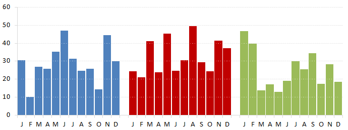
The final chart:


The lines may be a little thin for your tastes, just adjust the line weight until you get the effect you are trying to achieve.

I hope you enjoy the post and that you find something of value in it.

Additional resources:
How do you use the SeriesCollection in your VBA or work with series in your charts? Let us know in the comments below.


Points Of Interest

0

Hello World! (Sorry, I could not resist J) I was recently asked by our host, Jordan, if I would be interested in being a guest author here at Option Explicit VBA. I quickly and humbly accepted. I will strive to do my best to add something of value. Let’s dive right in.

I was inspired the other day by Chandoo’s post on his blog in regards to tax burden as well as Jared’s subsequent submission regarding service levels. Both charts use a consistent color across what appears to be different series in panel charts that are arranged closely together.

In fact, they are not, the area charts are one series with blank rows or columns inserted in the data range to create the separated effect. Here is a sample initial column chart I created using the same concept


So far, so good - but I would like each "Series" to have a different color. I selected some data points and changed the fill color


Looking good, but I'll need to manually select an additional 22 data points and change the fill color for each point. It gets worse if I want to add additional, "Series" to the chart or decide to go back and change a color - more manual work!

So I thought to myself, "Self, there must be an easier way!" The good news is that there is an easier way through VBA! Let's cook up some code (Option Explicit VBA - Remember?)

I only have one ChartObject with one SeriesCollection, so that part is straight forward. But there are many points in the SeriesCollection to be considered. Additionally, I dont want to plot anyting or add color to anything for points 13 and 25 where I have blank rows in my data.

So, I want to do something with points 1-12, 14-25, 27-38. Sounds like a good candidate for a Select Case..Case..End Select structure.


Option Explicit
1: Sub ColorDataPoints()
2: Dim wb As Workbook
3: Dim ws As Worksheet
4: Dim i As Integer
5: Dim lBlue As Long
6: Dim lRed As Long
7: Dim lGreen As Long
8: Set wb = ThisWorkbook
9: Set ws = wb.Worksheets("Sheet2")
10: lBlue = RGB(79, 129, 189)
11: lRed = RGB(192, 0, 0)
12: lGreen = RGB(155, 187, 89)
13: With ws
14: For i = 1 To .ChartObjects(1).Chart.SeriesCollection(1).Points.Count
15: Select Case i
16: Case 1 To 12
17: .ChartObjects(1).Chart.SeriesCollection(1).Points(i).Interior.Color = lBlue
18: Case 14 To 25
19: .ChartObjects(1).Chart.SeriesCollection(1).Points(i).Interior.Color = lRed
20: Case 27 To 38
21: .ChartObjects(1).Chart.SeriesCollection(1).Points(i).Interior.Color = lGreen
22: End Select
23: Next i
24: End With
25: 'Tidy up
26: Set ws = Nothing
27: Set wb = Nothing
28: End Sub


Now I have a chart with one x-axis and what appears to be 3 different series, when in fact, it is one. Perhaps more importantly, I have a process that requires very little updating as my needs change to display more "Series" or to change colors.

More on the Points Collection.

Download the workbook .

How do you work with points in your charts and VBA? Let us know in the comments section.


Details on Demand: Bring up details on a graph with Excel rollovers

4
So, as usual, I've been experimenting more with the rollover technique. Last night, I started experimenting with adding the capability to rollover a point on a chart (instead of just a worksheet cell) to see if I could have a label appear - or just some event fire - upon the mouse entering a chart's datapoint's "hotspot." The goal was to improve upon previous attempts to provide details-on-demand for charts. Such attempts usually required that you create a reference to a chart object and use chart sheets. Personally, I don't like chart sheets.

In the end, I moved beyond just firing an event when your mouse hovers over a data point; instead, I created the functionality to select a rectangle of data points to display information about them. See:

Unable to display content. Adobe Flash is required.

Because I'm now writing a book, I don't really have time to go through what I did at length. But here's a short summary.

1. I first made every cell into a square of the same size, which you can learn how to do by reading my "Most Squares Method."

2. With each cell the same size, I now had a grid that I could turn into"hot spots" for the mouse rollover. I laid out my chart to use 36 (0 - 35) squares horizontally and 17 (0 - 16) vertically. There was really no good reason for why I picked these numbers; my choice was pretty arbitrary. However, for this method, the more squares you use, the more hotspots you create; thus, more squares means more precision.

3. I then created a mouse rollover technique to capture the row and column numbers set above. Using these numbers, I mapped them on to the charts grid (so for row two, I would do 2/17 * y-axis value to get an approximate mapping). With these mapping I could approximate where the hotspots would light up certain points that were within them

4. I didn't want the user to be able to click on the graph and change its values. So I took a shape and placed it on top of the graph and assigned it to fire a macro on click. You can't see the shape because the fill color is fully transparent. Reread that last sentence and note that I did not say I used "no fill color." When you assign a macro to a shape, if you select "no fill," Excel lets you select anything that is contained by the shape as if it's not there. That would mean the user would be able to select the graph, which is exactly what I didn't want. For the shape above, I simply set its transparency to 100%.

5. Finally, to make a long story short, the shape when clicked fires the macro that allows the user to draw the rectangle.

I know right now my work isn't perfect (some data points aren't selectable for example depending upon where you start the rectangle), but I like what I have now and don't have much more time to work on it. I'll leave it to you to put it to good use.

Let me know if you make something cool.

Download File
Details on Demand Rollover.xlsm


Needs More Rollover: Quick Tip!

2
More people are interested in Excel mouse rollovers, which I think is great. I'm especially enthusiastic about Chandoo's latest dashboard contest where I found out that several contestants used the technique! By the way, there are many great dashboards showcased in the contest. Take a look and make sure to vote!

So here's the tip. If you're familiar with the rollover method - and you should be by now, it's like all I ever blog about these days - you may have noticed that while your mouse is over a cell, Excel is continuously firing the rollover method. For example, let's take a look at this snippet from Chandoo's blog:

Public Function highlightSeries(seriesName As Range)
Range("valSelOption") = seriesName.Value
End Function


If you place your mouse over the cell with the HYPERLINK formula that calls this function, the range valSelOption will be continuously written to. This becomes a problem when there's a lot of complex interaction on your spreadsheet. If, for example, you've used a lot of volatile functions (like OFFSET or VLOOKUP), continuously writing to the sheet will mean a recalculation for each cell with the volatile function. Nobody likes a slow spreadsheet. 

The incredibly simple fix to our problem comes from the wonderful book, Professional Excel Development, by  Bullen, Bovey, and Green in their chapter on spreadsheet optimization and speed tricks. Simply test if you're rewriting the same value over and over again:

Public Function highlightSeries(seriesName As Range)
If Range("valSelOption") <> seriesName.Value Then Range("valSelOption") = seriesName.Value
End Function


In the above code, I test if valSelOption already equals seriesName.Value. If it does, then we do nothing; if not, we write to it so that the next time the function is called with the same value in its argument (which is unpreventable if your mouse is over a cell for even a brief moment second), we can again, relax and do nothing.

Thats it! You'll likely see an immediate speed improvement, especially if you're doing lots of complex stuff with your rollover, like a this.

Turn Off Cell Background Error Checking with VBA

3
When I'm all done with my Excel application, I'll usually want to flip off background error checking - that is, I'll tell Excel to stop showing those little green triangles that appear in cells. Don't get me wrong, those little green alerts can be useful - but they are rarely so in a finished product where I know my layout and formulas are correct. I just want to tell Excel, "thanks for the help, but stop annoying me already!" Indeed, these green alerts appeared on other computer screens when users opened my Periodic Table of elements file, which I found annoying.

The problem is that while I can tell those green triangles to go away on my instance Excel by going into Excel Options (or simply by clicking "ignore"), that won't fix the problem when my file is loaded onto other computers. The way around this is some VBA and the workbook open and close events. 

So, in my ThisWorkbook object in the VBA window, I wrote this:

Option Explicit

Private Sub Workbook_Open()
    Application.ErrorCheckingOptions.BackgroundChecking = False
End Sub

Private Sub Workbook_BeforeClose(Cancel As Boolean)
    Application.ErrorCheckingOptions.BackgroundChecking = True
End Sub

There are actually several types of background error checking that go on in a workbook. Excel allows you to disable these separate error checks by themselves if don't want to disable everything. Specifically, you can modify background checking options for empty cell references, error calculations, inconsistent formulas, and omitted cells, among others. For example, you might simply write:

Application.ErrorCheckingOptions.OmittedCells = False

if you only want Excel to stop monitoring for formula patterns that appear to omit cells that Excel thinks should be included in the formula. This will work so long as BackgroundChecking is still True. If you set BackgroundChecking to False like in the example above, Excel will cease all attempts to second guess your work (which can make your life easier, sometimes). 

To read more, see:

Interactive Periodic Table of Elements in Excel

46
I've been on a real rollover kick lately. I'm really trying to figure out if it can be useful. Earlier today I started making a Periodic Table of Elements using Excel. I employed the rollover technique to allow the user to gain information about an element simply by rolling over a cell. Well, for some reason, I couldn't stop there. So what was meant to be a small project ballooned into something larger. Unfortunately, my sticking to good coding practice didn't keep up with craving to do more. So what I present to you below isn't really a polished product. If you poke through the named ranges and the rollover indexes, you'll probably see that I add and subtract one to them somewhat randomly (a cheap trick - this is  due to my trying to reconcile the table copied from Wikipedia with my indices).

As you can see below, you can not only gain information about an element but you can also toggle on and off different element groupings.

Unable to display content. Adobe Flash is required.

If you want to "crack" the file, the first thing you'll need to do is reset the ScrollArea (Click on a cell. Go to the Developer tab, click Properties. Delete the reference in the ScrollArea box.). Then just unhide everything.

Good luck.
Periodic Table.xlsm

Update -
Reader Dario found an error in the spreadsheet (see the comments) - this is the result of some carelessness and cheap tricks on my part. An updated version will be released tonight. In the meantime however, you can still poke around the file :).

Another Update -
I've since fixed the bug described in the reader comments. If you find anything else, let me know!

How to: highlighting cells using the rollover technique in Excel

8
In my last post I used my patented rollover technique to create an effect similar to the one shown below:

Unable to display content. Adobe Flash is required.

Neat, huh? When you place your mouse over a cell, it changes color to show that you are selecting it. It's a true "rollover": no mouse-clicks required. In my last post, I show how that might be useful.

Wondering how I did it? Checkout this file:
Rollover Surprise.xlsm

Rollovers for Gantt Charts

2
Before we start, you might have noticed some renovations on this blog. Yeah, it was time for a change. I'm working this template out, so sorry if some of the formats seem off. Also, I have started a new facebook page. I'll be keeping it updated with stories from my favorite blogs. Also, you can post questions and stuff for me (or others) to take a crack at. Plus, you'll see that I'm just a normal average guy. So if you have a facebook, you should join. You really don't have a good excuse why not! :)

DOOOOOOOOOOOOO IT!
Option Explicit VBA | Promote Your Page Too


***

In early last year, this humble blog had very little traffic. All of that changed in April of last year when I posted an exciting discovery: the Rollover technique. This technique was written about by the wonderful Purna of Chandoo.org. At the time, I was super excited about all of the possibilities of this technique. Now, just about a year later, I'm unsure whether anyone (besides me) has really ever used it. I even tried to incorporate it into my last project, but I found my clients were all too used to clicking on a cell rather than rolling over one. In the end I removed the rollover and replaced it with a click. Perhaps the rollover technique is destined to be a cool gimmick and not much more.

But I'm not giving up. Reader Bert van Zandbergen has been sending me many fine spreadsheets featuring this technique. His enthusiasm is encouraging. So I give you a rollover you can use for your Gantt Charts!
Unable to display content. Adobe Flash is required.

Download the fun, here:
Gantt Chart Surprise.xlsm

To see my intermediate table, scroll to the right of the dashboard. Sometime in the short future, I'll post a how to make the highlighted cell stand out with a border. In the mean time, remember to go to Facebook and like this page. Seriously, what are you waiting for? 

Miscellaneous Stuff

1
First, a big thank you to everyone following my blog. Here's some stuff I'd like to share in no particular order.

Stephen Colbert Come to My Wedding


We (my fiance and I) want Stephen Colbert to come to our wedding, which is in October of this year. My beautiful and wonderful fiance explains as follows:
During the tedious processes of inviting people to our wedding, my fiance and I began a running joke of inviting Stephen Colbert. Well, he may still be joking, but I'm not.
We don't have terminal illnesses or a terribly romantic love story--unless you consider our burning desire to have Stephen Colbert at our wedding an illness and online dating terribly romantic.


Want to help? Of course you do! Do this:
(1) Like us on Facebook.
(2) Follow us on twitter
(3) Get your friends to do the same!
Thanks in advance for the help, internet - you're so awesome!

* * *

Excel Custom Formats

Lately, I've really been into Excel custom formatting. This is my favorite page to reference when I have questions about custom formatting: http://www.ozgrid.com/Excel/CustomFormats.htm

Make to checkout all the other info ozgrid has to offer!

Looking for a cool Excel forum?

I am a contributor to the Excel forum, Excel Heros on LinkedIn. This forum is associated with the terrific Excel Hero website.

Visualization and You

I have a lot of strong feelings about visualizations as you may have noticed in a previous blog post. I believe that many organizations, including the media, software companies, and even universities are encouraging meaningless and distorted data representations.

The visualization guru, Stephen Few, has this excellent quiz to test your Graph Design IQ. Check it out!

Right now, I'm reading Few's book, Now you see it, which I highly recommend. A link for it will be up later on an "excel resources" page when it's complete.

Want to hire an Excel consultant, but don't know where to begin?

This page from Daily Dose of Excel is a good place to start.

Let's join forces!

As you may have noticed, sometimes my blog updates are sparse. I do this in my spare time and sometimes I'm just too busy to update. Part of the problem is I start writing tutorials that always become too big. For example, I wanted my sensitivity analysis tutorial to be complete in one post -- already, it might grow to three or four! I have a real problem.

Do you like writing? More specifically, do you like writing on Excel? Want to join forces? I would really love to have some more regular posts. Drop me a line if you're interested!

Have just one post you think you might want to share? Again, drop me a line!

I'd love to hear from you

Comment below, email, facebook, twitter, LinkedIn... whatever you want. Have something interesting? Share it!

Guest Post #1 - Dynamic Funnel Chart

0
Reader, Bert van Zandbergen, from Beekbergen, The Netherlands (Holland) sent me his own cool creation based on the Rollover technique I created. I asked if I could post his work to this blog to which he graciously agreed.

Below is his write up. Some of the Excel functions below are in Dutch (which I think is really cool). If you're confused, download the file first - your version of Excel will show the functions in your language of choice. And, of course, if this technique is new to you, read the the tutorial on how to do Excel rollovers. 

***

Dynamic Funnel Chart

by
Bert van Zandbergen
The Netherlands

Based on this file: 
Figure 1
Start with the 4 columns. The dummy had to be 100 or more for space to unfilled dummy bars. Delete the lines. Now you can change the value from “100” to “1”. Further information is visible in Figure 1.

Hyperlink:
Read also the information and explanation on the website of Chandoo.org
http://chandoo.org/wp/2011/07/20/interactive-dashboard-using-hyperlinks/ 

Figure 2
Place a hyperlinks in the cells of the hotspot – see above. 

Figure 3
Formula: Define the hotspot with the name: “ valSelOption” 

Figure 4
Go to VBA and insert a module. For more information about the instruction – see on this website, the Chandoo website and the module above. 

Figure 5 -- Chart with hotspot
The hotspot is based on 10 columns combined with 42 rows. – see figure 5/6. The hotspots are linked by hyperlinks with corresponding cells in columns AI:AR.  For a special effect and an easy crossover the values are placed in a diagonal figure

See: Figure 5/6  
Figure 5 -- The "hotspot"

Above the hotspots and the linked cells. Special formed to make an easy crossover.

***

A big thank you to Bert - hopefully there will be more contributions in the future!

Do you have something interesting to share? Send me an email or drop me a line on LinkedIn. 

Edit button, please

3
This is a long overdue article, my apologies.

The basis of the article surrounds a question in the comments section of an article on Chandoo.org (comment #75) written about the hyperlink() method I discovered and wrote about here. In Chandoo’s example, when a user rolls over different “hotspots” representing different datasets, the corresponding data comes into view on a graph below. In other words, the rollover technique tells Excel to change the data currently being fed into the chart. One of the respondents to his post attempted an associated technique that would create a dynamic hyperlink to the dataset. The goal, essentially, was to create an “edit” button that could bring the user to the dataset in view.

The problem he (and I) ran into was that whenever we updated the link in the Hyperlink formula, the hyperlink's friendly name, “Edit,” would be replaced by the address of the actual link. This resulted in an Edit hyperlink that read something like “Sheet!A1” instead of “Edit Sales.” While the link worked, the result was ugly. We needed to try something different.

So here's my solution. It’s nothing really fancy, but it does require you to keep track of two components: (1) the tab that holds your associated data; and (2) the beginning cell of your associated data. There are, indeed, many ways to keep track of this information, but some planning and organization helps out a lot. One of the easiest organization techniques is to have your data in the same cell for each tab. If your “Sales” data begins in cell B1, then any other data you'd like to use for this technique should also start in B1. Moreover, if you're interested in information from your sales tab, name your tab “Sales” (and your other tabs “expenses,” “income,” etc.).  Similarly, if you are pulling from different databases, tab one could be Database1, tab two Databse2, etc. Alas, not all data can be organized in this manner, but you get the picture. Such organization makes a significant difference when implementing this technique and my example below assumes you have data from tabs Database1, Database2, and Database3.

A Quick Refresher


The dashboard above works the same way as the example used in Chandoos’ post. The cell’s with the down arrows are the rollover hotspots and they contain the required hyperlink formulas.


For example, when the user places his or her mouse of cell B5, C5, or D5 the following code is executed.

Public Function ChangeSelection(i As Integer)
     Range("valSelOption") = i

End Function


Hopefully this is all review for you. If not – or, for a quick refresher – read these:
1. Rollover b8 ov1
2. Interactive Dashboard in Excel using Hyperlinks

On to the Good Stuff

So now we need a button that, when clicked, will take us to the location where the data resides. As you might have noticed from my example above, I placed a textbox on my dashboard with the label “Edit.” This is my edit “hyperlink.” But instead of actually “hyperlinking” to the data, I’ll instead tell Excel to take me to the data with a macro. In my module I’ve written the following code and have assigned it to the textbox.


Public Sub GoToData()

Dim wsCurrent As Excel.Worksheet
Set wsCurrent = Worksheets("Database" & Range("valSelOption"))
wsCurrent.Activate
wsCurrent.Range("B2").Activate
End Sub


Here’s what’s going on. In the earlier code section – my ChangeSelection function – I told excel to change the named range, valSelOption, to an index representing the location where my data resides. But I’ve also named my tabs Database1, Database2, and Database3. Since I placed my data starting in range B2 for each tab, I can use valSelOption to direct Excel to the correct tab. In the above code, I create a worksheet object and assign it to the correct worksheet by concatenating “Database” with valSelOption. In other words, if I valSelOption is 1, then the database we want will be Database1...and so forth.

Also, notice that my code first activates the tab we want before activating the range within it.  This is an important step that must come first or you will surely get an error.

---

So what if your data isn't organized in an easy, uniform way? Well, in my example, you might change cells B3 to D3 to the name of your tabs. And in your ChangeSelection() function you would have a string argument instead of an integer. That could help your program identify the tab housing your data. Again there are different ways to do this.

But if you find that your data is all over the place – consider reorganizing!

-

(I’ll have the file up with this example soon.)

My Top 5 VBA Development Environment Tips

2
So you've got a project that requires VBA – you’re ready and excited – and you jump right in! But here come the headaches! With every syntax error the visual basic environment interrupts your programming mojo with an annoying popup. You remembered to place comments in your code – but where are the ones you’re looking for? When did Excel programming become so frustrating?

Below, I’ll describe how I've customized my editor to minimize annoyance and maximize efficiency. It might not help you become a better programmer…but then again, it really might! Your best work probably comes from a space you can call your own. So season your VBA developer environment to taste.

Tip #1: Change the Font
The problem is that the default font, Courier New, does a poor job differentiating between colors - especially when your eyes quickly scan the screen. Don’t believe me? See the difference for yourself with my personal font choice: Consolas, 9pt.

Go to Tools > Options, then click on the “Editor Format” tab to try out a new font. Whatever you choose, you’ll need to keep these things in mind:
  • You want a font that makes a significant contrast between colors.
  • You want a fixed-width font. If you choose a font that is not fixed-width, you’ll have trouble using Tab to align your code. Some well known fixed-width fonts are: Consolas and Lucida Console.
  • Pick something readable. Stay away from Mistrel.

Tip #2: Change your Comment Formatting
Make a statement with bold comments! Seriously though, the default comment formatting blends right in with the rest of the code. And that’s a pain – especially, when you’re on the hunt for some code you had commented to save for later.  I like my comments with a light-blue highlight in the background and a dark-blue foreground. They really stand out.

Go to Tools > Options, then click on the “Editor Format.” Select “Comment Text” from the list to get started.

Tip #3: Use the Immediate window, immediately
The Immediate window should be your best friend, but some folks didn’t even know it exists. Go to View > Immediate window if it’s not already open.

Why is it so great? Well, the immediate window allows you to print essential information to the screen while your program is running. Let’s say you need to iterate through tons of data and would like to know your intermediate progress but only temporarily. You can print to the immediate window by using Debug.Print(). Go ahead, try Debug.Print “foo!” in a Sub.

But wait, there’s more: you can also gain information even when you’re not running anything. Go place a shape onto an empty spread sheet and make sure you’ve selected it. Now go to your Immediate window and type Msgbox Selection.Width. Hit Enter.

Is your UserForm stuck in an endless loop? (it happens sometimes) Do a CTRL+Break and type “Unload Me” into the Immediate window to return everything to normal.

Tip #4: No more syntax error pop-ups
Sometimes you’re typing an IF/THEN but see some code above it that needs fixing. You click-off to go fix the code but you’re stopped by an annoying popup message. I mean, it’s nice of VBA to let you know there’s an error, but it didn’t need to ruin your flow.

So get rid of those nasty pop-ups by going to Tools > Options and unchecking Auto Syntax Check. The environment will still tell you that you have an error by highlighting the offending script in red - but the pesky popup box will bother you no more.

Tip #5: Opt for Option Explicit By putting Option Explicit at the top of your code, you are helping yourself so much. Seriously, I’m such an advocate of Option Explicit that I named my blog after it.

What does it do? It requires that you declare your variables. If you don’t write "Dim i as integer,” you will not be allowed to use i for anything. Without explicit declaration, VBA assumes that any new variable introduced is a variant type.

Explicit declaration might sound like more work, but trust me you’ll save yourself some headache. You’ll find that you might not always spell your variables correctly, for example, “RecordCount” might accidently be spelled as “RecrodCount.” When your program doesn’t give the correct output (because it assumes “RecrodCount” is actually a new variable), you’ll be forced to scour through your code looking for the problem, which you might not even realize is a typo. And if you missed the typo when you first typed it out, it’s likely that your quick scanning will miss it again. By requiring explicit declaration, undeclared variables will result in a runtime error, so you can fix your variables before they become hidden within your code.

Don’t make Option Explicit optional. Go to Tools > Options and proudly check “Require Variable Declaration.”


Your developing environment is just as important and personal as any other. Make sure you use the features and options within the Visual Basic Environment to customize to the fullest.

One Size Fits All

30
Anyone who has a made a dashboard in Excel before has probably experienced this problem: a dashboard that fits nicely on your screen but not so nicely on your client’s. Yes, it’s the age old problem of differing monitors, resolutions, font-sizes and other settings that make what looks great on your screen look too small or too big on another’s. I’ve seen a few ideas to get around this problem that include resizing the spreadsheet controls to resizing the Excel window. Here’s my idea.

Most likely, your current Dashboard is already zoomed to its “best view.” By that I mean your current spreadsheet is at the proper zoom level such that your dashboard is displayed most effectively. If it’s not, go ahead and set it to the optimal zoom for your screen. Use the picture below as a guide for your dashboard and adjust the zoom levels (down in the lower-right corner) accordingly.


In this next step you’ll want to take note of the columns spanning your screen. Above, you’ll see that I’ve selected columns “A1:Z1,” but left the final column, “AA1” unselected. I would suggest highlighting all except for the last column as I did above—when we are finished, the last column will act as a nice margin. Jot down your selection; we’ll be using it in a moment.

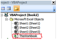
Fire up the Visual Basic editor. Since we want our Dashboard to be in the correct view whenever someone opens the file (otherwise, what’s the use?) we’re going to add some code to be executed right when the workbook is first opened. In the upper-left hand corner of the Visual Basic Editor you’ll see a box labeled Project, which contains your Microsoft Excel objects. Double click ThisWorkbook—the workbook object belonging to our project.


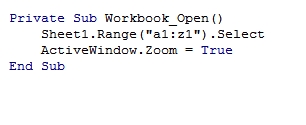
In the code window, select “Workbook” from the object dropdown on the left. Then select the “Open” method from the method dropdown on the right. The Workbook_Open() procedure should appear on the screen as shown below.


Now enter the following code into your new procedure. Remember the range I said to jot down for later? Use that range in the quotes as I have for “A1:Z1.”
Now to see if our code actually works! Go back to the spreadsheet and, for testing purposes, zoom really far out to a level that your dashboard should never go. Now save and quit. (Make sure you save it as a .xlsm macro enabled workbook.)

Open your dashboard! Neat, huh? If you want to make your dashboard super snazzy, take the row selection you jotted down above and do Merge and Center on it. Now add a nice title to it for a nifty dashboard banner.

---

There are a few things I should mention. The user might have to hit “Enable Macros” before the code takes effect, but there’s not a ton you can do about that. And if Excel wasn’t closed correctly on a previous use, that box showing unsaved files will most likely appear and your dashboard, left with less screen real estate, will probably not zoom correctly. Finally, sometimes Excel will not open to a maximized state – but you can fix this with some VBA code.

I’ve found this to be a good workaround in my projects– but I haven’t worked with every different client computer, either. Let me know what you guys think – was this useful? How do you get around displaying the same thing on different screens?

Completing the Square aka The "Most" Squares Method

0
Now that I actually have some traffic to this blog, it's probably time I started adding posts.

A while ago, I was wondering how to make the cells in Excel exactly square, like the squares on graph paper.  I came across this post from Mr. Excel.  I wasn't in love with his solution because it requires users to first find their desired width by dragging a column, then writing it down (keep in mind it's in pixels, so you might not have an easy round number), and then entering it into an input box.

So, without further ado, I present my solution that doesn't require you to write anything down:

Private Sub AutoSize()

    Dim cels As Range
    Set cels = Me.Cells
 
    cels.ColumnWidth = 1  'Adjust me
    cels.RowHeight = cels(1, 1).width
 
    Set cels = Nothing

End Sub

To get different sized squares, simply adjust your ColumnWidth.  For further reading, checkout why widths in Excel are so tricky.

How to Create a Rollover Effect in Excel: Execute a Macro When Your Mouse is over a Cell

362
"Rollover B8 OV1" (like Rollover Beethoven...? get it?)

Update 17 July 2011: This blog entry was featured in Chandoo's latest post. So if you're coming here from his site -- welcome!

original post:
This post was inspired by Chandoo's post on hyperlinks in Excel. If you haven't checked his website out yet - you should. It's excellent.

In this post, I suggest a method for creating a "Rollover" effect for your mouse on an Excel spreadsheet. Rollover techniques (also called "Mouseovers") are useful to (1) display quick information to the user; (2) to execute a function when a user puts their mouse over a specific region; and (3) to make neat graphical effects.

For item 1, my technique isn't really necessary. If you want to display brief information to the user when he or she rolls over a cell, the best way to do this is to insert a comment.

But comments are pretty limited. You can only write so much information in a comment before it becomes too cluttered to be useful. Moreover, comments are static. What if you want the information concerning the "target" cell (that is, the cell to be rolled over) to change based on different items in your spreadsheet? We can use the in-cell Hyperlink() formula to accomplish this.

The Hyperlink() formula looks like this:

=Hyperlink(location, [Friendly Text])
location - Here you write the intended address of your hyperlink. This can be a webpage (i.e. "http://www.google.com") or a file on your computer.
[Friendly Text] - This is an optional field that provides a caption to your hyperlink. If you leave it blank, it will simply display the address in the previous parameter.

To begin our example, you'll need to create a User Defined Function (UDF) to be executed when the rollover event is initiated. So go into the Visual Basic Environment, create or find a free module and create a UDF that looks something like this.

Public Function MyMouseOverEvent()
Sheet1.Range("A1").Value = "Event Fired!"
End Function
I can understand if you're puzzled at this point. UDFs are not really allowed to change values in other cells. However, since we'll be calling this function from within the Hyperlink() formula, you'll see this limitation no longer exists.

So now go to Sheet1 and click on cell A2. In that cell, type in the following formula:

=HYPERLINK(MyMouseOverEvent(),"Click here")
Upon hitting Enter, you should get a #VALUE! error, but ignore it for a second. Roll your mouse over cell A2 - and viola! - Cell A1 should now say "Event Fired!"

But what about that pesky #VALUE! error? Remember the limitation that UDFs can't change other cells? Well, even though Excel let's you change a value from within your UDF, it still recognizes that it wasn't supposed to! To get rid of that error is pretty simple. Just rewrite the function in your cell as follows:

=IFERROR(HYPERLINK(MyMouseOverEvent(),"Click here"), "Click here")

And that's it. If you like this technique and find some cool uses for it, drop me an email and show me.

Here's some graphical fun I created using this technique. Putting the mouse inside the black rectangle creates a fading snake-like pattern based on your mouse movements. Check out the screen capture:


Make sure to check out my latest (and greatest) example of this technique, here:

Getting a Handle on hWnd

4
Sometimes, you'll want to programmatically take advantage of Windows outside the capabilities readily available through Visual Basic for Applications (VBA). For example, both eliminating the "Close"-button or creating a more opaque background on a window require the use of the Windows API.

Doing this in Visual Basic isn't too hard, but there are some distinct differences between what's readily available to programmers in Microsoft Office's Visual Basic (VBA) compared to its virtual twin, Visual Basic 6.0, and its smarter, object-oriented younger brother VB.net. Specifically, UserForms in VBA do not contain methods to find their Windows handle, (aka, their hWnd).

And most window modifying APIs require the target window's handle. Luckily, the Windows API also contains a function to find a given window's hWnd, called FindWindow():


Public Declare Function FindWindow Lib "user32" Alias "FindWindowA" _
(ByVal lpClassName As String, ByVal lpWindowName As String) As Long


So, to find your window's handle, you'll do something like this (assuming you're coding within the UserForm).


hWnd = FindWindow("ThunderDFrame", me.caption)


Here, FindWindow() takes two arguments. First, the class name of the window for which you're searching; and second, the window's caption.

ThunderDFrame, huh?

I know, right? The UserForms in Excel are actually of the Windows class ThunderDFrame, which is the class for all UserFroms in Microsoft Office applications after 2002 (it was "ThunderXFrame" before that). I've looked online for a good explanation for the name but haven't really found anything. Either way you'll need to pass that into the first argument of FindWindow whenever you need a UserForm's handle.


That's all for now!

-

ps I'm working on a better stylesheet for when I display code.