46

I've been on a real rollover kick lately. I'm really trying to figure out if it can be useful. Earlier today I started making a Periodic Table of Elements using Excel. I employed the rollover technique to allow the user to gain information about an element simply by rolling over a cell. Well, for some reason, I couldn't stop there. So what was meant to be a small project ballooned into something larger. Unfortunately, my sticking to good coding practice didn't keep up with craving to do more. So what I present to you below isn't really a polished product. If you poke through the named ranges and the rollover indexes, you'll probably see that I add and subtract one to them somewhat randomly (a cheap trick - this is  due to my trying to reconcile the table copied from Wikipedia with my indices).

As you can see below, you can not only gain information about an element but you can also toggle on and off different element groupings.



If you want to "crack" the file, the first thing you'll need to do is reset the ScrollArea (Click on a cell. Go to the Developer tab, click Properties. Delete the reference in the ScrollArea box.). Then just unhide everything.

Good luck.
Periodic Table.xlsm

Update -
Reader Dario found an error in the spreadsheet (see the comments) - this is the result of some carelessness and cheap tricks on my part. An updated version will be released tonight. In the meantime however, you can still poke around the file :).

Another Update -
I've since fixed the bug described in the reader comments. If you find anything else, let me know!

Author: Unknown Labels: Advanced Excel, Data Visualizations, Dynamic Charts, Formulas, Interactive Dashboards, Rollovers, Spreadsheet Tricks, VBA

11

Anyone who has used a Form Control Label likely knows its limitations: you can't increase the font-size, -color, or style.  Below, you can see that these formatting items have been "grayed out" in the Font group on the Excel Ribbon.

To be sure, the Label control has received a lot of flack for these deficiencies.  A look through some Excel forums shows suggestions to use a TextBox shape or an ActiveX Label instead of the hapless Label control.It's a tragedy since the other form controls are lightweight and easy to use. Some forum posters even said Labels are best used to cover cells you don't want the user to click. So sad.   

But things are looking up.  I've since discovered you can take a boring Label Control from this...

...to this!

How?

As it turns out, Labels take on the text-font and -size features of a referenced cell.  So, to make my label look this this, I simply linked it to a pre-formatted cell, like G2, below.

In fact, this is the same mechanism to link a Textbox shape to a cell.  The difference here is that a Textbox can take an unformatted cell and apply new formatting on the front-end, when it's displayed to the user.  Above, we see that the cell must first be formatted, then linked.  In fact, whatever formatting exists in the cell when you first make the link, the label will maintain this format until a new link is created.  For example, if I were to change G2 to a black color and a smaller font, the label would not show these new changes (however, it would change its text if I changed the value in G2 to something else).  So to change the Label's formatting -- even when it's linked to the same cell -- you'll need to click the label, click the formula bar, and retype the cell link.  

Admittedly, everyone else might have already figured this one out.  However, I'm still very excited.  Don't get me wrong, Textbox Shapes are great, but having too many could become expensive on your spreadsheet, especially if you are constantly updating the screen (how many redraws can your computer handle before things start to slow?).  Labels, as Form Controls, inherently carry less bloat and overhead.  They're perfect for dynamic dashboards.  

Author: Unknown Labels: Excel Tricks, Formulas, No VBA, Pivot Tables

0

Excel really doesn't have an explicit "between function" to allow users, given a set of ranges, to find in what range a selected number falls. The obvious and messy workaround is to use a bunch of nested IFs, which is tedious and error-prone. That's where the RANK function comes in.

Here's a breakdown.

RANK(number,ref,[order])
number - The number you want to find
ref - The reference to spreadsheet range
order - optional; excel defaults to descending order

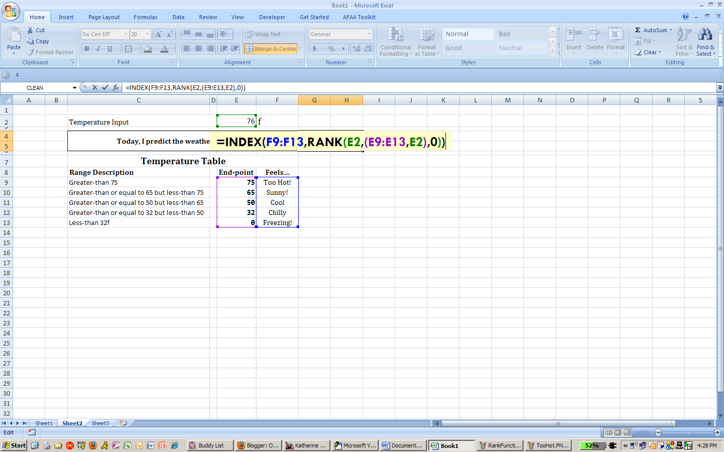
The RANK function returns the location of a specified number in a given range. So let's say you have a given set, 1,2,3,4,5. Obviously, testing for the number three will return a location of 3. For our range test, we combine a number outside the set and see where it falls.

Check out the image below to see it in action:


Excel returns a rank of 4, since 3.2 will appear in the fourth location of the ranked set, 1,2,3,3.2,4,5.
At this point, there are two important items to point out.

• How excel sorts the data for ranking is important. Above we use an ascending order (we pass a 1 to the last argument) and below we'll use a descending order (we'll pass a 0 to the last argument). You'll have to decide which best fits your analysis.
• Because you combine two ranges into one, you must use parenthesis. If you miss this step, the RANK function will interpret B2 as the next parameter and return an error.

Here's a Weather Application



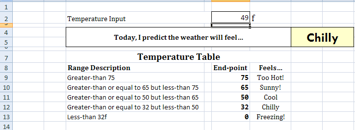
This example tests for a temperature's range and then displays how the day will feel corresponding to that range.

-

You could also use this trick when you must evaluate a value on a complex function. For example, you might have a graph with several curves that represents some utility for a given value, x. Thus, if you know the bounds of your curves, you can test in what range your x falls and apply its corresponding curve-function.

Finally, you might have noticed that this trick restricts you to inequalities with an inclusive lower bound and exclusive upper bound. There's ways to fix this and I plan to talk more about them in future posts.

Author: Unknown Labels: Excel Math, Formulas, Lookups, Rank()