Everyone! We've moved to WordPress.

Investigations in "Illegal Activities" with User Defined Functions

0
A group of fellow Excel experts who call themselves the Frankens Team were encouraged by the rollover method to investigate other known instances in which Excel has allowed for the impossible; namely, allowing UDFs to change the value of other cells.

I invite everyone to view their terrific analysis: Excel formula to change the value of another cell?

Also, take a look around the site (which is mostly in Italian - so get that Google translator ready!) for some great Excel stuff, like Creative and advanced chart design in Excel.

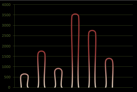
By the way, what would you call this type of chart?

Courtesy E90E50 fx
:)

The Excel Rollover Mini FAQ

26
As more people are use the rollover method (or “Interactive Hyperlinks” as Chandoo calls them), I thought it might be helpful to answer common questions I've seen popping up on forums. So, in no particular order, I present the Excel Rollover Mini FAQ!

1. Are there example articles and spreadsheets on how to use Excel rollovers?


Here’s a list: 
Articles and Tutorials
How to Create a Rollover Effect in Excel: Execute a Macro When Your Mouse is over a Cell by Me
How to: highlighting cells using the rollover technique in Excel by Me
Interactive Dashboard in Excel using Hyperlinks by Chandoo
Needs More Rollover: Quick Tip! by Me
Une macro sensible à la souris by Monsieur Excel (this one is in French!)
Handling Rollover Clicks Without Using the Worksheet_SelectionChange Event by Me
Roll Over Tooltips and Web Actions on a Microsoft Excel Dashboard by Robert Mundigl of ClearlyAndSimply.com
Guest Post: Rollover for Months and Years by Bert van Zandbergen (klvzndbrgn (at) gmail )
Dynamic Funnel Chart by Bert van Zandbergen
If you know of others or would like me to add an informative article you've written, go ahead and email me a link. 

2. Do rollovers work in Excel 2003 and in versions previous?

No, I don't think so. I haven't tested this for myself, but comments on other blogs suggest that the method only works for versions 2007 and 2010. Excel 2013 is not yet out, so while I think it will work in that version, we will have to wait and see for ourselves.

[updated 9/21/2012]

Maybe. I might have been wrong about what I said earlier. You see, I've always used IFERROR to surround the HYPERLINK formula, but I forgot IFERROR didn't exist for Excel until version 2007. This formula by Zoran Stanojević might conceivably work in Excel 2003:

=REPT("",ISERROR(HYPERLINK(getCoordinates(....),"")))


Additionally, Zoran writes:

I always avoid version specific functions when they are unnecessary because they potentially weakening the universal solution.

That's an incredibly good point. Still, I'm probably not going to give up IFERROR anytime soon :).

But, if you are you are employing the rollover method on your own spreadsheet--and you're concerned with backward compatibility issues--definitely consider using his formula above. Then come back and share the results with your good buddy, Jordan.

Also, I had an email conversation with someone recently who attempted to run my introduction to the rollover method file, "Snakey", in Excel 2013 preview. He said the file eventually crashed Excel 2013. However, it was the preview version, so whether the rollover method works in the final version still remains to be seen.  For this blog's sake, I hope the rollover method works correctly in Excel 2013.

3. Why/how do rollovers work? I thought User Defined Functions could not change other values on a spreadsheet. I've also heard this functionality doesn't exist in Excel.

As far as I can tell the rollover method shouldn't exist. I think it works by taking advantage the Hyperlink formula in a way unforeseen by the original developers. Intentional or not, the functionality I believe has opened a door to some cool new possibilities with Excel. 

I can only speculate why rollovers work the way they do. My best guess is that when your mouse floats over a hyperlink, Excel goes out behind the scenes to check if the hyperlink exists and loads the address in memory in anticipation of a click. This piece of memory probably goes into a generic callback procedure which knows how to handle the different actions that fill the callback queue. Because a User Defined Function is supplied instead of a URL or reference on the spreadsheet (as is normally the case when use Hyperlink) the callback function treats the UDF like any other and executes it immediately without knowing that it came from the Hyperlink formula. 

I could be wrong about all of this, but that's my (rather uneducated) guess. If any of you know better, I welcome your feedback. If I'm wrong, let me know. My feelings won't be hurt. 

4. Is there a way to handle multiple rollovers on the same sheet?

Yes. Simply create another rollover function in your module and point it to the new rollover function in your module. As far as I can tell, there is no limit to how many rollovers your spreadsheet can employ at any given time.  

5. When my mouse is over the hyperlink, Excel continuously fires the macro which is slowing everything down. Is there anything I can do about this? 

Yep, try this.

6. I want the entire cell to become a rollover hotspot, but the user defined function only fires when my mouse is on the text of the hyperlink - how can I make the entire cell a hotspot?

Enable wordwrap in each cell containing the rollover method.

7. My rollovers used to work perfectly, but now they don't work at all! Recently I added some formulas like INDEX, VLOOKUP, and SUM to the hyperlink rollover formula. Now everything appears without error, but the macro no longer fires. What happened? I need to make my formulas dynamic!

Rollovers appear like regular formulas but they are not. When you add other formulas to them, they tend to not work as planned (they may work if you select the cell and hit Enter - but that's not what you want). However, you can make your rollover functions dynamic, but you cannot do it by adding formulas directly to the rollover formula. 

Here's what's I've found. Apparently, rollover formulas work exactly like references used for dynamic charts, dynamic labels, and form controls. Let's take the chart example. When you want to make a dynamic chart, you must have your chart series refer to a range containing the dynamic data. You can't place an INDEX function directly into your chart's SERIES function, but you can have your chart point to a set of data that uses the INDEX function. You'll have to create the same mechanism when using rollovers. So, if you want to make your hyperlink formula change its "friendly text" based something the user does, place a reference to the range with your dynamic content in the friendly text parameter of the HYPERLINK formula and the return error parameter of your IFERROR formula. 

It's really no different than what you would do when working with a dynamic chart. But unlike in charts and form controls - Excel won't give you a warning when you've placed stuff into the rollover formula that shouldn't be there - instead, your rollovers just won't work. 


8. How do I handle clicks on my Rollover cells?

You can use the Worksheet_SelectionChange event, but I prefer this method.

9. Do rollovers work on non-Windows machines, like Macs?

I don't think so. Rollovers require Visual Basic for Applications and the latest versions of Office for Macs don't include the ability to create or run macros, from what I'm told. 

If you're a mac user and have success using the rollover method, I'd certainly love to hear from you about it.

Can I add to this list?

Sure! Email me or post thoughts, examples, advice, etc. 
Turn Off Cell Background Error Checking with VBA

3
When I'm all done with my Excel application, I'll usually want to flip off background error checking - that is, I'll tell Excel to stop showing those little green triangles that appear in cells. Don't get me wrong, those little green alerts can be useful - but they are rarely so in a finished product where I know my layout and formulas are correct. I just want to tell Excel, "thanks for the help, but stop annoying me already!" Indeed, these green alerts appeared on other computer screens when users opened my Periodic Table of elements file, which I found annoying.

The problem is that while I can tell those green triangles to go away on my instance Excel by going into Excel Options (or simply by clicking "ignore"), that won't fix the problem when my file is loaded onto other computers. The way around this is some VBA and the workbook open and close events. 

So, in my ThisWorkbook object in the VBA window, I wrote this:

Option Explicit

Private Sub Workbook_Open()
    Application.ErrorCheckingOptions.BackgroundChecking = False
End Sub

Private Sub Workbook_BeforeClose(Cancel As Boolean)
    Application.ErrorCheckingOptions.BackgroundChecking = True
End Sub

There are actually several types of background error checking that go on in a workbook. Excel allows you to disable these separate error checks by themselves if don't want to disable everything. Specifically, you can modify background checking options for empty cell references, error calculations, inconsistent formulas, and omitted cells, among others. For example, you might simply write:

Application.ErrorCheckingOptions.OmittedCells = False

if you only want Excel to stop monitoring for formula patterns that appear to omit cells that Excel thinks should be included in the formula. This will work so long as BackgroundChecking is still True. If you set BackgroundChecking to False like in the example above, Excel will cease all attempts to second guess your work (which can make your life easier, sometimes). 

To read more, see:

Guest Post #1 - Dynamic Funnel Chart

0
Reader, Bert van Zandbergen, from Beekbergen, The Netherlands (Holland) sent me his own cool creation based on the Rollover technique I created. I asked if I could post his work to this blog to which he graciously agreed.

Below is his write up. Some of the Excel functions below are in Dutch (which I think is really cool). If you're confused, download the file first - your version of Excel will show the functions in your language of choice. And, of course, if this technique is new to you, read the the tutorial on how to do Excel rollovers. 

***

Dynamic Funnel Chart

by
Bert van Zandbergen
The Netherlands

Based on this file: 
Figure 1
Start with the 4 columns. The dummy had to be 100 or more for space to unfilled dummy bars. Delete the lines. Now you can change the value from “100” to “1”. Further information is visible in Figure 1.

Hyperlink:
Read also the information and explanation on the website of Chandoo.org
http://chandoo.org/wp/2011/07/20/interactive-dashboard-using-hyperlinks/ 

Figure 2
Place a hyperlinks in the cells of the hotspot – see above. 

Figure 3
Formula: Define the hotspot with the name: “ valSelOption” 

Figure 4
Go to VBA and insert a module. For more information about the instruction – see on this website, the Chandoo website and the module above. 

Figure 5 -- Chart with hotspot
The hotspot is based on 10 columns combined with 42 rows. – see figure 5/6. The hotspots are linked by hyperlinks with corresponding cells in columns AI:AR.  For a special effect and an easy crossover the values are placed in a diagonal figure

See: Figure 5/6  
Figure 5 -- The "hotspot"

Above the hotspots and the linked cells. Special formed to make an easy crossover.

***

A big thank you to Bert - hopefully there will be more contributions in the future!

Do you have something interesting to share? Send me an email or drop me a line on LinkedIn. 

Change the Font Size, Color, and Style of an Excel Form Control Label

11
Anyone who has used a Form Control Label likely knows its limitations: you can't increase the font-size, -color, or style.  Below, you can see that these formatting items have been "grayed out" in the Font group on the Excel Ribbon.


To be sure, the Label control has received a lot of flack for these deficiencies.  A look through some Excel forums shows suggestions to use a TextBox shape or an ActiveX Label instead of the hapless Label control.It's a tragedy since the other form controls are lightweight and easy to use. Some forum posters even said Labels are best used to cover cells you don't want the user to click. So sad.   

But things are looking up.  I've since discovered you can take a boring Label Control from this...


...to this!


How?

As it turns out, Labels take on the text-font and -size features of a referenced cell.  So, to make my label look this this, I simply linked it to a pre-formatted cell, like G2, below.


In fact, this is the same mechanism to link a Textbox shape to a cell.  The difference here is that a Textbox can take an unformatted cell and apply new formatting on the front-end, when it's displayed to the user.  Above, we see that the cell must first be formatted, then linked.  In fact, whatever formatting exists in the cell when you first make the link, the label will maintain this format until a new link is created.  For example, if I were to change G2 to a black color and a smaller font, the label would not show these new changes (however, it would change its text if I changed the value in G2 to something else).  So to change the Label's formatting -- even when it's linked to the same cell -- you'll need to click the label, click the formula bar, and retype the cell link.  

Admittedly, everyone else might have already figured this one out.  However, I'm still very excited.  Don't get me wrong, Textbox Shapes are great, but having too many could become expensive on your spreadsheet, especially if you are constantly updating the screen (how many redraws can your computer handle before things start to slow?).  Labels, as Form Controls, inherently carry less bloat and overhead.  They're perfect for dynamic dashboards.  


Truncating Long Text to Fit into Cells

5
Have you had a list of names but found your cell width too small to show every name?  Take a look at this:


I had my nonexistent secretary print out this fake itinerary for me.  Nothing lines up neatly.  Look how some of my events overlap the cell boundary between columns B and C.  My 2012 End-of-world Steering Committee meeting on February 1st, 2013 goes long and is then cut-off by the date!

To fix this, you could have Excel automatically size Column B, but that's a bit unpredictable to have on a dashboard (what if other content is sized off the screen?).  We'll just have to accept that we can't show everything, but we can make it look neater.  We'll employ some type of text truncation method similar to what Microsoft uses to display the names of files in Windows Explorer: if the text to be displayed is greater than a certain character length, simply truncate and add a "...".

The "Original Recipe" Method

First thing we'll need to do is figure out how many characters we'll want to display before truncation.  There's really no way to do this without trial and error. But, to make life easier, we can use =LEN("Your Text Here") to return the length of your text; or, we can use something like  =LEFT(B3, 4) to return the first four characters of text in cell B3.  Keep trying until you find a good character length.  

Hopefully, you got a good handle on using LEN and LEFT above because we'll be using them from here on out.  Also, I'm going to use 25 characters as my desired character length before truncation.  Below I use  LEFT to pull the first 25 characters from each event name.


Now we'll need to know which names to add the "..." to.  Following ExcelHero's discussion on using IFs, we'll avoid using one here; not to worry, we don't really need it.

As it turns out, LEFT can take a zero value character length -- it just returns nothing.  So to have Excel automatically return what we want, we'll do this:

=LEFT("…",LEN(B3)>25)

Take a look at that second argument on the right.  It takes the length of our event name and tests if it's greater than our cutoff length of 25.  If it's less than 25, Excel will return a zero and display nothing.  If it's greater than the cutoff, Excel will return a 1 and display the first character in our text.  But there's something I found out while writing this tutorial, I expected Excel to only return one period ("."), but instead it returns all three ("...") even if you only put a 1 in on the right.  I'm guessing that the ellipses are treated as one character; however, I'm dubious that this works in every case on every computer, so to have your formula return three characters or zero, you'll simply change it to:

=LEFT("…",(LEN(B3)>25) * 3)

Now you'll need to concatenate both strings together using the concatenation operator, &.


Finally, as you can see in cell, H7, there is a space between the event name and the ellipses.  This is because the last character before the cutoff was a space.  To fix this, surround the first string formula with the TRIM function; this will automatically delete any leading or ending spaces.  

Putting it all Together

To finish, we'll combine all our steps into one formula, like so:

=TRIM(LEFT(B3,25)) & LEFT("…",LEN(B3)>25)

To get:
...mmmmmmuch better!

Download my example: Spillover Design Example.xlsx

Edit button, please

3
This is a long overdue article, my apologies.

The basis of the article surrounds a question in the comments section of an article on Chandoo.org (comment #75) written about the hyperlink() method I discovered and wrote about here. In Chandoo’s example, when a user rolls over different “hotspots” representing different datasets, the corresponding data comes into view on a graph below. In other words, the rollover technique tells Excel to change the data currently being fed into the chart. One of the respondents to his post attempted an associated technique that would create a dynamic hyperlink to the dataset. The goal, essentially, was to create an “edit” button that could bring the user to the dataset in view.

The problem he (and I) ran into was that whenever we updated the link in the Hyperlink formula, the hyperlink's friendly name, “Edit,” would be replaced by the address of the actual link. This resulted in an Edit hyperlink that read something like “Sheet!A1” instead of “Edit Sales.” While the link worked, the result was ugly. We needed to try something different.

So here's my solution. It’s nothing really fancy, but it does require you to keep track of two components: (1) the tab that holds your associated data; and (2) the beginning cell of your associated data. There are, indeed, many ways to keep track of this information, but some planning and organization helps out a lot. One of the easiest organization techniques is to have your data in the same cell for each tab. If your “Sales” data begins in cell B1, then any other data you'd like to use for this technique should also start in B1. Moreover, if you're interested in information from your sales tab, name your tab “Sales” (and your other tabs “expenses,” “income,” etc.).  Similarly, if you are pulling from different databases, tab one could be Database1, tab two Databse2, etc. Alas, not all data can be organized in this manner, but you get the picture. Such organization makes a significant difference when implementing this technique and my example below assumes you have data from tabs Database1, Database2, and Database3.

A Quick Refresher


The dashboard above works the same way as the example used in Chandoos’ post. The cell’s with the down arrows are the rollover hotspots and they contain the required hyperlink formulas.


For example, when the user places his or her mouse of cell B5, C5, or D5 the following code is executed.

Public Function ChangeSelection(i As Integer)
     Range("valSelOption") = i

End Function


Hopefully this is all review for you. If not – or, for a quick refresher – read these:
1. Rollover b8 ov1
2. Interactive Dashboard in Excel using Hyperlinks

On to the Good Stuff

So now we need a button that, when clicked, will take us to the location where the data resides. As you might have noticed from my example above, I placed a textbox on my dashboard with the label “Edit.” This is my edit “hyperlink.” But instead of actually “hyperlinking” to the data, I’ll instead tell Excel to take me to the data with a macro. In my module I’ve written the following code and have assigned it to the textbox.


Public Sub GoToData()

Dim wsCurrent As Excel.Worksheet
Set wsCurrent = Worksheets("Database" & Range("valSelOption"))
wsCurrent.Activate
wsCurrent.Range("B2").Activate
End Sub


Here’s what’s going on. In the earlier code section – my ChangeSelection function – I told excel to change the named range, valSelOption, to an index representing the location where my data resides. But I’ve also named my tabs Database1, Database2, and Database3. Since I placed my data starting in range B2 for each tab, I can use valSelOption to direct Excel to the correct tab. In the above code, I create a worksheet object and assign it to the correct worksheet by concatenating “Database” with valSelOption. In other words, if I valSelOption is 1, then the database we want will be Database1...and so forth.

Also, notice that my code first activates the tab we want before activating the range within it.  This is an important step that must come first or you will surely get an error.

---

So what if your data isn't organized in an easy, uniform way? Well, in my example, you might change cells B3 to D3 to the name of your tabs. And in your ChangeSelection() function you would have a string argument instead of an integer. That could help your program identify the tab housing your data. Again there are different ways to do this.

But if you find that your data is all over the place – consider reorganizing!

-

(I’ll have the file up with this example soon.)

My Top 5 VBA Development Environment Tips

2
So you've got a project that requires VBA – you’re ready and excited – and you jump right in! But here come the headaches! With every syntax error the visual basic environment interrupts your programming mojo with an annoying popup. You remembered to place comments in your code – but where are the ones you’re looking for? When did Excel programming become so frustrating?

Below, I’ll describe how I've customized my editor to minimize annoyance and maximize efficiency. It might not help you become a better programmer…but then again, it really might! Your best work probably comes from a space you can call your own. So season your VBA developer environment to taste.

Tip #1: Change the Font
The problem is that the default font, Courier New, does a poor job differentiating between colors - especially when your eyes quickly scan the screen. Don’t believe me? See the difference for yourself with my personal font choice: Consolas, 9pt.

Go to Tools > Options, then click on the “Editor Format” tab to try out a new font. Whatever you choose, you’ll need to keep these things in mind:
  • You want a font that makes a significant contrast between colors.
  • You want a fixed-width font. If you choose a font that is not fixed-width, you’ll have trouble using Tab to align your code. Some well known fixed-width fonts are: Consolas and Lucida Console.
  • Pick something readable. Stay away from Mistrel.

Tip #2: Change your Comment Formatting
Make a statement with bold comments! Seriously though, the default comment formatting blends right in with the rest of the code. And that’s a pain – especially, when you’re on the hunt for some code you had commented to save for later.  I like my comments with a light-blue highlight in the background and a dark-blue foreground. They really stand out.

Go to Tools > Options, then click on the “Editor Format.” Select “Comment Text” from the list to get started.

Tip #3: Use the Immediate window, immediately
The Immediate window should be your best friend, but some folks didn’t even know it exists. Go to View > Immediate window if it’s not already open.

Why is it so great? Well, the immediate window allows you to print essential information to the screen while your program is running. Let’s say you need to iterate through tons of data and would like to know your intermediate progress but only temporarily. You can print to the immediate window by using Debug.Print(). Go ahead, try Debug.Print “foo!” in a Sub.

But wait, there’s more: you can also gain information even when you’re not running anything. Go place a shape onto an empty spread sheet and make sure you’ve selected it. Now go to your Immediate window and type Msgbox Selection.Width. Hit Enter.

Is your UserForm stuck in an endless loop? (it happens sometimes) Do a CTRL+Break and type “Unload Me” into the Immediate window to return everything to normal.

Tip #4: No more syntax error pop-ups
Sometimes you’re typing an IF/THEN but see some code above it that needs fixing. You click-off to go fix the code but you’re stopped by an annoying popup message. I mean, it’s nice of VBA to let you know there’s an error, but it didn’t need to ruin your flow.

So get rid of those nasty pop-ups by going to Tools > Options and unchecking Auto Syntax Check. The environment will still tell you that you have an error by highlighting the offending script in red - but the pesky popup box will bother you no more.

Tip #5: Opt for Option Explicit By putting Option Explicit at the top of your code, you are helping yourself so much. Seriously, I’m such an advocate of Option Explicit that I named my blog after it.

What does it do? It requires that you declare your variables. If you don’t write "Dim i as integer,” you will not be allowed to use i for anything. Without explicit declaration, VBA assumes that any new variable introduced is a variant type.

Explicit declaration might sound like more work, but trust me you’ll save yourself some headache. You’ll find that you might not always spell your variables correctly, for example, “RecordCount” might accidently be spelled as “RecrodCount.” When your program doesn’t give the correct output (because it assumes “RecrodCount” is actually a new variable), you’ll be forced to scour through your code looking for the problem, which you might not even realize is a typo. And if you missed the typo when you first typed it out, it’s likely that your quick scanning will miss it again. By requiring explicit declaration, undeclared variables will result in a runtime error, so you can fix your variables before they become hidden within your code.

Don’t make Option Explicit optional. Go to Tools > Options and proudly check “Require Variable Declaration.”


Your developing environment is just as important and personal as any other. Make sure you use the features and options within the Visual Basic Environment to customize to the fullest.
