3

Make sure to checkout A Dynamic Dashboard for Project Durations and Costs in Excel (part 2) for the example file!

Let’s say you are the manager of a portfolio of projects at your company.  While each project under your aegis is different, they have a few things in common; specifically – and for the sake of our example – they all go through (or, are currently in) three different phases, and each phase has a different cost per month, but the cost doesn’t differ between each project.  In our example, the phases are:

Phase Name Cost of each stage per month
1. Planning $250/month
2. Execution $500/month
3. Maturity $125/month

The idea is to capture both the cost in any given month and the overall cost over the life of the project.  For example, you have an IT Upgrades project in your portfolio.  You think that you will spend two months in Planning, nine months in Execution, and one month in Maturity after which the project will be closed.  Thus, the overall cost of your project is expected to be,

Planning @ two months: 2 months * $250 $/month  = $500
Execution @ nine months: 9 months * $500 $/month = $4500
Maturity @ one month: 1 month * $125 $/month = $125
Planning + Execution + Maturity =  $500 + $4500 + $125 = $5125

The problem is that each project is different.  One project might spend more time in the first phase than the other.  Moreover, for some projects you have a good idea of how long they will stay in each phase, and for some you are a bit less sure.  Boy, you say, wouldn't it be nice to change how long a project stays in each phase to compare costs.  Wouldn't it be nice to see it on a chart?  Let's see what we can do.

Using a VLOOKUP might seem like an obvious choice for our solution.  Here's how to do it.   

The Dynamic VLOOKUP Method

Step 1: Create the VLOOKUP table
Since you know there are three projects, you could encode ids into a lookup table numbers as follows.

Step 2: Create a Reference Table
The Reference Table is a time-series table that holds the numerical references to your VLOOKUP table.  If IT Services has two months of Planning, then the Reference Table will show two 1's in the first two months, respectively.

Step 3: Create a Values Table to map each reference to its monthly cost using VLOOKUP
Now, you'll make another table that is essentially a mirror image of your Reference Table. This table, however, maps each reference to the correct cost.  So, for Month 1 in the Values Table, VLOOKUP will use the corresponding reference (1) in the Reference Table to indicate the project is in the Planning phase and the associated cost is $250.

Step 4: Sum the Values Table, then graph

Summary
Our dynamic VLOOKUP() method works: the manager (that's us) can replace the values in the Reference Table to update how long a project stays in each phase.  We would simply repeat numbers in the Reference Table in the amount of months a project is in a particular phase.  Our Values Table automatically updates based on each change.



So here's the thing.  I don't like this method at all.  For one, we need a VLOOKUP in for every month, for every program.  Our example only displayed a few projects in a small time frame, but the real world might have many projects over many years!  That's a real problem because VLOOKUPs can become computationally expensive as our spreadsheet grows.

And there's another problem, too.  The manager – that's us, remember – must hand-jam the references in for every month. What if there are many years to account for?  We could Copy/Paste to make life easier, but this method is so very, very error-prone.  There should be a way for us to simply enter the months a project is in a given phase and have Excel automatically generate all the required reference information.

Let's talk about how to do that in the next post.

If you're having trouble with the work above, take some time to see if you can recreate your own version in Excel.  Even if you have followed everything so far, consider the VLOOKUP method and the importance of using numeric references.  They will play a very key role in part 2. 


-----


Now Available: A Dynamic Dashboard for Project Durations and Costs in Excel (part 2)

Author: Unknown Labels: Dashboards, Dynamic Charts, No VBA, Project Management

1

Most importantly, use your words
An ideal Excel filename should be two or three succinct words and contain few numbers. Current operating systems no longer constrain filename character length, so there is neither excuse for nor cleverness in using shorthand. Capitalize each word as you would a document title.    

Only abbreviate proper nouns
If your file is an example to someone, it should have the full word “Example” not “ex” in its title. If your Excel dashboard is the second version of the “Cost Analysis and Reporting System” you may abbreviate your filename to “CARS v2.xlsx,” but a VBA Chart Tutorial should never be named “VB ChrtTut.xlsm.”

Always connect words with a space and nothing else
The name of your file is not a programming variable or engineering quantity. The words in your filename should not be connected with underscores (“_”) nor dashes (“-“).

Use clear dates, but don’t include dates in every filename
Unless your file is a report that comes out on a specific, periodic schedule, there’s likely not a good reason to put today’s date in your filename. If you must put a date in your file, place the date at the beginning, left-hand side of the filename so it appears first. This ensures the date is not cut off when viewed in a file explorer. Dated files are likely to be stored with similar files in the same folder, so cutting off the last bit of each filename on the right is less harmful than cutting off the date.

If the workbook is a monthly report, the name should by the three character month followed by the year, then another space for the filename (e.g. “May 2012 Cost Report”). For reports that occur more frequently, a MM-DD-YYYY is preferable for sorting within the file directory.  \However, dates must always be clear; do not write “03-12” as this could mean March 12 or March 2012. Finally, full dates should not be clumped together without a dash (bad: “03122012”).

Numbers are preferable to dates
If you have several iterations of a file, use a numbering system instead of dates. Using dates leads to the horrible practice of adding extra numbers at the end of the filename. For example: “InventoryList 22 Feb 2001_1.xlsx”, “InventoryList 22 Feb 2001_2.xlsx” … etc.  Moreover, using dates and the former practice will not instantly make clear the latest version of your file when viewed in a file directory. However, placing a number at the end of your filename (“Inventory List 1.xlsx”, “Inventory List 2.xlsx”) always will make clear the latest (and first) iteration of the file whether sorted by filename, file type, or date modified when viewed in a directory (these files will always be either first or last). Numbers always should appear as the last character on the right.

Author: Unknown Labels: Excel Standards, Filename

3

This is a long overdue article, my apologies.

The basis of the article surrounds a question in the comments section of an article on Chandoo.org (comment #75) written about the hyperlink() method I discovered and wrote about here. In Chandoo’s example, when a user rolls over different “hotspots” representing different datasets, the corresponding data comes into view on a graph below. In other words, the rollover technique tells Excel to change the data currently being fed into the chart. One of the respondents to his post attempted an associated technique that would create a dynamic hyperlink to the dataset. The goal, essentially, was to create an “edit” button that could bring the user to the dataset in view.

The problem he (and I) ran into was that whenever we updated the link in the Hyperlink formula, the hyperlink's friendly name, “Edit,” would be replaced by the address of the actual link. This resulted in an Edit hyperlink that read something like “Sheet!A1” instead of “Edit Sales.” While the link worked, the result was ugly. We needed to try something different.

So here's my solution. It’s nothing really fancy, but it does require you to keep track of two components: (1) the tab that holds your associated data; and (2) the beginning cell of your associated data. There are, indeed, many ways to keep track of this information, but some planning and organization helps out a lot. One of the easiest organization techniques is to have your data in the same cell for each tab. If your “Sales” data begins in cell B1, then any other data you'd like to use for this technique should also start in B1. Moreover, if you're interested in information from your sales tab, name your tab “Sales” (and your other tabs “expenses,” “income,” etc.).  Similarly, if you are pulling from different databases, tab one could be Database1, tab two Databse2, etc. Alas, not all data can be organized in this manner, but you get the picture. Such organization makes a significant difference when implementing this technique and my example below assumes you have data from tabs Database1, Database2, and Database3.

A Quick Refresher

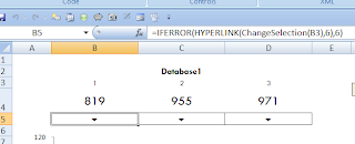
The dashboard above works the same way as the example used in Chandoos’ post. The cell’s with the down arrows are the rollover hotspots and they contain the required hyperlink formulas.

For example, when the user places his or her mouse of cell B5, C5, or D5 the following code is executed.


Public Function ChangeSelection(i As Integer)
     Range("valSelOption") = i
End Function



Hopefully this is all review for you. If not – or, for a quick refresher – read these:
1. Rollover b8 ov1
2. Interactive Dashboard in Excel using Hyperlinks

On to the Good Stuff

So now we need a button that, when clicked, will take us to the location where the data resides. As you might have noticed from my example above, I placed a textbox on my dashboard with the label “Edit.” This is my edit “hyperlink.” But instead of actually “hyperlinking” to the data, I’ll instead tell Excel to take me to the data with a macro. In my module I’ve written the following code and have assigned it to the textbox.


Public Sub GoToData()


Dim wsCurrent As Excel.Worksheet
Set wsCurrent = Worksheets("Database" & Range("valSelOption"))
wsCurrent.Activate
wsCurrent.Range("B2").Activate

End Sub


Here’s what’s going on. In the earlier code section – my ChangeSelection function – I told excel to change the named range, valSelOption, to an index representing the location where my data resides. But I’ve also named my tabs Database1, Database2, and Database3. Since I placed my data starting in range B2 for each tab, I can use valSelOption to direct Excel to the correct tab. In the above code, I create a worksheet object and assign it to the correct worksheet by concatenating “Database” with valSelOption. In other words, if I valSelOption is 1, then the database we want will be Database1...and so forth.

Also, notice that my code first activates the tab we want before activating the range within it.  This is an important step that must come first or you will surely get an error.

---

So what if your data isn't organized in an easy, uniform way? Well, in my example, you might change cells B3 to D3 to the name of your tabs. And in your ChangeSelection() function you would have a string argument instead of an integer. That could help your program identify the tab housing your data. Again there are different ways to do this.

But if you find that your data is all over the place – consider reorganizing!

-

(I’ll have the file up with this example soon.)

Author: Unknown Labels: Dashboards, Dynamic Charts, Excel Tricks, VBA

2

So you've got a project that requires VBA – you’re ready and excited – and you jump right in! But here come the headaches! With every syntax error the visual basic environment interrupts your programming mojo with an annoying popup. You remembered to place comments in your code – but where are the ones you’re looking for? When did Excel programming become so frustrating?

Below, I’ll describe how I've customized my editor to minimize annoyance and maximize efficiency. It might not help you become a better programmer…but then again, it really might! Your best work probably comes from a space you can call your own. So season your VBA developer environment to taste.

Tip #1: Change the Font
The problem is that the default font, Courier New, does a poor job differentiating between colors - especially when your eyes quickly scan the screen. Don’t believe me? See the difference for yourself with my personal font choice: Consolas, 9pt.

Go to Tools > Options, then click on the “Editor Format” tab to try out a new font. Whatever you choose, you’ll need to keep these things in mind:

• You want a font that makes a significant contrast between colors.
• You want a fixed-width font. If you choose a font that is not fixed-width, you’ll have trouble using Tab to align your code. Some well known fixed-width fonts are: Consolas and Lucida Console.
• Pick something readable. Stay away from Mistrel.

Tip #2: Change your Comment Formatting
Make a statement with bold comments! Seriously though, the default comment formatting blends right in with the rest of the code. And that’s a pain – especially, when you’re on the hunt for some code you had commented to save for later.  I like my comments with a light-blue highlight in the background and a dark-blue foreground. They really stand out.

Go to Tools > Options, then click on the “Editor Format.” Select “Comment Text” from the list to get started.

Tip #3: Use the Immediate window, immediately
The Immediate window should be your best friend, but some folks didn’t even know it exists. Go to View > Immediate window if it’s not already open.

Why is it so great? Well, the immediate window allows you to print essential information to the screen while your program is running. Let’s say you need to iterate through tons of data and would like to know your intermediate progress but only temporarily. You can print to the immediate window by using Debug.Print(). Go ahead, try Debug.Print “foo!” in a Sub.

But wait, there’s more: you can also gain information even when you’re not running anything. Go place a shape onto an empty spread sheet and make sure you’ve selected it. Now go to your Immediate window and type Msgbox Selection.Width. Hit Enter.

Is your UserForm stuck in an endless loop? (it happens sometimes) Do a CTRL+Break and type “Unload Me” into the Immediate window to return everything to normal.

Tip #4: No more syntax error pop-ups
Sometimes you’re typing an IF/THEN but see some code above it that needs fixing. You click-off to go fix the code but you’re stopped by an annoying popup message. I mean, it’s nice of VBA to let you know there’s an error, but it didn’t need to ruin your flow.

So get rid of those nasty pop-ups by going to Tools > Options and unchecking Auto Syntax Check. The environment will still tell you that you have an error by highlighting the offending script in red - but the pesky popup box will bother you no more.

Tip #5: Opt for Option Explicit By putting Option Explicit at the top of your code, you are helping yourself so much. Seriously, I’m such an advocate of Option Explicit that I named my blog after it.

What does it do? It requires that you declare your variables. If you don’t write "Dim i as integer,” you will not be allowed to use i for anything. Without explicit declaration, VBA assumes that any new variable introduced is a variant type.

Explicit declaration might sound like more work, but trust me you’ll save yourself some headache. You’ll find that you might not always spell your variables correctly, for example, “RecordCount” might accidently be spelled as “RecrodCount.” When your program doesn’t give the correct output (because it assumes “RecrodCount” is actually a new variable), you’ll be forced to scour through your code looking for the problem, which you might not even realize is a typo. And if you missed the typo when you first typed it out, it’s likely that your quick scanning will miss it again. By requiring explicit declaration, undeclared variables will result in a runtime error, so you can fix your variables before they become hidden within your code.

Don’t make Option Explicit optional. Go to Tools > Options and proudly check “Require Variable Declaration.”


Your developing environment is just as important and personal as any other. Make sure you use the features and options within the Visual Basic Environment to customize to the fullest.

Author: Unknown Labels: Excel Development, Excel Tips, Excel Tricks, Programming, Spreadsheet Tricks, VBA

30

Anyone who has a made a dashboard in Excel before has probably experienced this problem: a dashboard that fits nicely on your screen but not so nicely on your client’s. Yes, it’s the age old problem of differing monitors, resolutions, font-sizes and other settings that make what looks great on your screen look too small or too big on another’s. I’ve seen a few ideas to get around this problem that include resizing the spreadsheet controls to resizing the Excel window. Here’s my idea.

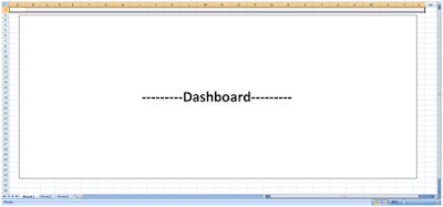
Most likely, your current Dashboard is already zoomed to its “best view.” By that I mean your current spreadsheet is at the proper zoom level such that your dashboard is displayed most effectively. If it’s not, go ahead and set it to the optimal zoom for your screen. Use the picture below as a guide for your dashboard and adjust the zoom levels (down in the lower-right corner) accordingly.




In this next step you’ll want to take note of the columns spanning your screen. Above, you’ll see that I’ve selected columns “A1:Z1,” but left the final column, “AA1” unselected. I would suggest highlighting all except for the last column as I did above—when we are finished, the last column will act as a nice margin. Jot down your selection; we’ll be using it in a moment.

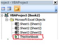
Fire up the Visual Basic editor. Since we want our Dashboard to be in the correct view whenever someone opens the file (otherwise, what’s the use?) we’re going to add some code to be executed right when the workbook is first opened. In the upper-left hand corner of the Visual Basic Editor you’ll see a box labeled Project, which contains your Microsoft Excel objects. Double click ThisWorkbook—the workbook object belonging to our project.




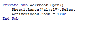
In the code window, select “Workbook” from the object dropdown on the left. Then select the “Open” method from the method dropdown on the right. The Workbook_Open() procedure should appear on the screen as shown below.



Now enter the following code into your new procedure. Remember the range I said to jot down for later? Use that range in the quotes as I have for “A1:Z1.”

Now to see if our code actually works! Go back to the spreadsheet and, for testing purposes, zoom really far out to a level that your dashboard should never go. Now save and quit. (Make sure you save it as a .xlsm macro enabled workbook.)

Open your dashboard! Neat, huh? If you want to make your dashboard super snazzy, take the row selection you jotted down above and do Merge and Center on it. Now add a nice title to it for a nifty dashboard banner.

---

There are a few things I should mention. The user might have to hit “Enable Macros” before the code takes effect, but there’s not a ton you can do about that. And if Excel wasn’t closed correctly on a previous use, that box showing unsaved files will most likely appear and your dashboard, left with less screen real estate, will probably not zoom correctly. Finally, sometimes Excel will not open to a maximized state – but you can fix this with some VBA code.

I’ve found this to be a good workaround in my projects– but I haven’t worked with every different client computer, either. Let me know what you guys think – was this useful? How do you get around displaying the same thing on different screens?

Author: Unknown Labels: Dashboards, VBA, Views, Zoom